What are parameter estimates even
People often try and estimate things. For example, people at tech companies tend to run a lot of experiments in order to estimate the impact of various policies (e.g. new website layout) on important-ish things (e.g. user signup rate). The process generally works like this:
- run your experiment and get some data
- use your data to build an estimate of the impact of your policy
- assume that this estimate is your best proxy for the true impact
- base your decisions on this estimate of the impact (e.g. move to the new website layout if the impact on conversion is sufficiently positive)
As it turns out, step 3 is actually not quite correct, and your estimate is in general not your best proxy for the true impact. I recently saw a presentation by Tom Cunningham and Dominic Coey from Facebook Research discussing their attempts at solving this problem. The intuition is straightforward but somewhat unintuitive (James-Stein), which leads to some interesting organizational challenges in practice. I’ll describe these things here.
Intuition
- Let \(\gamma\) be the true impact, and \(\hat{\gamma}\) be your estimate.
- If your experiment was designed correctly, then your estimate should just be the truth plus some uncorrelated noise: \begin{equation} \mathbb{E}[\hat{\gamma}\mid\gamma]=\gamma \end{equation}
- However, we don’t actually care about this quantity. Instead, what we want is the best estimate of \(\gamma\) given our estimate. That is: \begin{equation} \mathbb{E}[\gamma\mid\hat{\gamma}] \end{equation}
- In general, \(\mathbb{E}[\gamma\mid\hat{\gamma}] \neq \hat{\gamma}\), so we can probably do better than just using \(\hat{\gamma}\) as a proxy for the true value \(\gamma\).
That’s really all there is to it. From a Bayesian perspective this is quite clear. Your estimate is going to be the true value plus some noise: \(\hat{\gamma}=\gamma+\epsilon\), so conditional on the estimate \(\hat{\gamma}\), there’s some distribution of possible true \(\gamma\)s that could have generated this \(\hat{\gamma}\), and in general this distribution isn’t going to average out to exactly \(\hat{\gamma}\).
It’s worth noting a few things:
- This has nothing to do with endogeneity / your experiment being bad.
- This has nothing to do with selection bias / somehow only seeing large estimates / people exaggerating their effect sizes.
Probably shrink your estimates (but not always)
Alright, so your estimate \(\hat{\gamma}\) is going to be an imperfect proxy for the truth \(\gamma\). Most of the time, your estimate will be too extreme and will need to be shrunk down, but sometimes they’ll be too conservative and will need to be scaled up. Some examples to illustrate this:
1. Probably shrink your estimates
On average, your parameter estimates are going to be over-biased because of noise. Consider this example: let \(\hat{\gamma}=\gamma+\epsilon\) with \(\gamma\) and \(\epsilon\) mean-\(0\) and independent. If you fit a linear regression of \(\gamma\) on \(\hat{\gamma}\) \begin{equation} \gamma = a+b\hat{\gamma} \end{equation} then the coefficients \(a,b\) will be just \begin{equation} a=\mathbb{E}[\gamma]=0, \quad b = \frac{cov(\gamma, \hat{\gamma})}{var(\hat{\gamma})} = \frac{var(\gamma)}{var(\gamma)+var(\epsilon)}<1 \end{equation} That is, if you restrict yourself to just applying some uniform scaling to your estimates, then the best adjustment (in a squared loss sense) is to shrink your estimate towards the mean. The noisier your estimate is, the more you should shrink it. Even though \(E[\hat{\gamma}\mid\gamma]=\gamma\), you should still shrink it.
A few points:
- The mean-zero assumption is WLOG since you can just… demean everything.
- This is basically just attenuation bias / errors in variables.
- This is also basically just James-Stein.
We can go ahead and simulate this. We’ll assume all noise is Gaussian because that’s easy, though the above result doesn’t require any parametric assumptions.
import numpy as np
import matplotlib.pyplot as plt
%matplotlib inline
from sklearn.linear_model import LinearRegression

n = 1000
gamma = np.random.normal(size=n)
gamma_hat = gamma + np.random.normal(size=n)

lm = LinearRegression()
lm.fit(gamma_hat.reshape(-1,1), gamma)
print(lm.intercept_, lm.coef_)

plt.scatter(gamma_hat, gamma, alpha=.1)
xhat = np.linspace(gamma_hat.min(), gamma_hat.max(), 100)
yhat = lm.predict(xhat.reshape(-1,1))
plt.plot(xhat, yhat, color='red')
plt.xlabel('gamma_hat')
plt.ylabel('gamma')
plt.title('coefficient on gamma_hat: {:.3f}'.format(lm.coef_[0]))
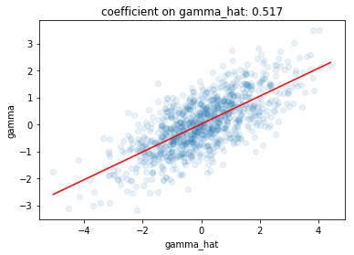
As expected, the coefficient on gamma_hat here is around 1/2 since the variance of the truth and the variance of the noise are equal.
2. But not always
So, on average, you should probably shrink down your estimates. But there are clear situations where you should scale them up instead. Consider this example:
- the distribution of true parameter value is bimodal
- your parameter estimate ends up being just below one of the modes
- thus, the true value is probably a bit closer to that mode than your parameter estimate
- so, you should probably scale your estimates up a bit
We can also go and simulate this, where we make the distribution of true parameter values a mixture of two Gaussians centered on either side of the origin. Thus, parameter estimates near 0 should be scaled up, whereas parameter estimates far from zero should be scaled down:
import numpy as np
import matplotlib.pyplot as plt
%matplotlib inline
from statsmodels.nonparametric.kernel_regression import KernelReg
from sklearn.linear_model import LinearRegression

n = 1000
loc = 3
gamma = np.concatenate([np.random.normal(loc=-loc, size=n),
                       np.random.normal(loc=loc, size=n)])
gamma_hat = gamma + np.random.normal(size=n*2)

kr = KernelReg(gamma, gamma_hat, var_type ='c', reg_type = 'lc', bw=[1])

plt.scatter(gamma_hat, gamma, alpha=.1)
xhat = np.linspace(gamma_hat.min(), gamma_hat.max(), 100)
yhat = kr.fit(xhat)[0]
plt.plot(xhat, yhat, color='red')
plt.xlabel('gamma_hat')
plt.ylabel('gamma')
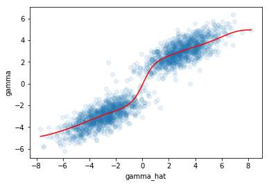
The slope of the local regression is quite high around 0, indicating that the estimates should be scaled up around 0, whereas further away from 0 the slope is lower.
What to do in practice?
Ok, so it seems like it might make sense to scale your parameter estimates up/down (mostly down). But how do you actually implement something like this in practice? If we could observe the true \(\gamma\) in addition to our estimates \(\hat{\gamma}\), then we could just try and estimate \(\mathbb{E}[\gamma\mid \hat{\gamma}]\) with some kind of regression like we did in the examples above. That’s too bad, because \(\gamma\) is clearly not observable, but the Facebook guys proposed a not unreasonable method for how to do this anyway:
- suppose you want to run an experiment
- break your population into two groups
- literally run the experiment twice in parallel on each of the two groups
- get two estimate of the true parameter from the two groups: \(\hat{\gamma}_1=\gamma+\epsilon_1\), \(\hat{\gamma}_2=\gamma+\epsilon_2\)
- do this every time you run any experiment
- take all of this data you have now, fit some kind of regression of \(\hat{\gamma}_1\) on \(\hat{\gamma}_2\)
- use your predicted value of \(\hat{\gamma}_1\) given \(\hat{\gamma}_2\) from your fitted regression as your best proxy for the true effect size
- use this predicted value to inform decisions instead of the raw estimates
Under the assumption that \(\epsilon_1\) and \(\epsilon_2\) are independent of each other and of \(\gamma\), then you have \begin{equation} \mathbb{E}[\hat{\gamma}_1\mid \hat{\gamma}_2] = \mathbb{E}[\gamma+\epsilon_1 \mid \gamma+\epsilon_2] = \mathbb{E}[\gamma\mid \hat{\gamma}_2] \end{equation} Which is exactly what we’re after. So if the errors are orthogonal then you can just do some regression to get the conditional expectation of one estimate on the other, which gives you the conditional expectation of the true parameter value given your estimate. For the most part, this makes a lot of sense. Some potential issues:
- The error terms \(\epsilon_1, \epsilon_2\) can be correlated because of e.g. common time shocks (as in, maybe all effect sizes are just randomly bigger during the summer). This would cause the \(\epsilon\)s to be correlated, and thus this conditional expectation to be more extreme than the truth: \(\lvert\mathbb{E}[\hat{\gamma}_1\mid\hat{\gamma}_2]\rvert > \lvert\mathbb{E}[\gamma\mid\hat{\gamma}_2]\rvert\).
- You’re breaking your sample in two, so if your experiment is about market-level dynamics that has weird scaling with size, then the half-size estimates won’t really be what you’re after.
Absent these issues, you can just do this two-sample split and use some estimate of \(\mathbb{E}[\hat{\gamma}_1\mid\hat{\gamma}_2]\) as your best proxy for the true effect \(\gamma\). So, literally do this 2-sample split procedure for every experiment, and then run some sort of local regression of \(\hat{\gamma}_1\) on \(\hat{\gamma}_2\), and use the predicted value from your regression instead of the raw estimates.
But of course, it’s not that simple…
Organizational challenges
In spite of the fairly clear reasons to not use your raw parameter estimate as a proxy for the true parameter value, this is literally what almost everyone does almost all the time. The fact that even for one of the largest and most sophisticated tech companies in the world, it’s literally the research group that is just now starting to figure out how to implement this should give you some indication of how widespread this practice is. Here are some potential reasons for why people use raw parameter estimates:
- This is just what people are taught. In academia, you generally report your parameter estimates, not some Bayesian posterior mean / some otherwise adjusted thing. So once people leave grad school, they continue doing this.
- It’s not entirely clear how to estimate \(\mathbb{E}[\hat{\gamma}_1\mid\hat{\gamma}_2]\).
- You can do a local regression, but there’s a lot of tuning parameters. How do you pick these? Or how do you stipulate a reasonable way to pick these?
- Why restrict to just conditioning on \(\hat{\gamma}_2\)? Why not do
\begin{equation}
\mathbb{E}[\hat{\gamma}_1\mid\hat{\gamma}_2, \text{ other stuff}]
\end{equation}
Surely there are other useful features that can be used to get even better proxies of the truth?- Estimates for certain sets of parameters (e.g. marketing-related things) might tend to be more exaggerated, whereas the reverse may be true for others (e.g. website layout). Should we include features controlling for this?
- Or, maybe experiments run during the winter tend to be less biased than those done in the summer? So maybe we should also condition on season?
- Maybe experiments run by engineers have effects that are less exaggerated than those run by product managers. Should we incorporate this feature?
- etc…
- And once you incorporate all of these things, how do you pick a method for computing this conditional expectation? How do you pick tuning parameters?
If you’re just one person doing some analyses, then you can maybe come up with something that does pretty ok for now. But when you’re in charge of designing a general process for how to adjust parameter estimates for a large institution, this problem becomes much harder. Here’s a speculative list of reasons:
- It’s fairly difficult to ex-ante specify the right way of resolving all of the various uncertainties in implementing some process like this. You’ll go along and realize you’ve forgotten some edge cases and have to fix stuff as they come up.
- Someone whose bonus depends on ‘succeeding’ on some metric is going to be unhappy you’re shrinking their estimate down, and they’ll argue with you that things should be done in some way that benefits them. So you’re going to have to spend a lot of time managing these conflicts.
- If there’s a significant number of people who aren’t happy with the policy, you’re going to have a hard time building the kind of cultural credibility to really establish some system like this.
- It might be pretty hard to measure/sell the impact of having improved parameter estimates to whomever is paying you, especially if you’re explicitly making life harder for many people in your organization.
- You might create perverse incentives where people will cheat on their experiments because if their estimates end up being bad, they’ll cause your regression to think that their entire group runs bad experiments, and thus anger their entire team / endanger their careers.
These problems are probably not insurmountable, but they certainly aren’t trivial to solve on an institutional level. So maybe it’s not so surprising that almost every place just goes with just the straight up raw parameter estimates. They might not be great, but they’re easy, and often it’s better to be fast and ballpark than slow and exact.